To program a CFD solver, you discretize the conservation equations on a mesh, couple pressure to velocity, solve the resulting linear systems iteratively, advance the solution in time and, from the first commit, test that each piece does what the mathematics says it should. The code is the easy part to describe. Demonstrating that it is correct is the hard part.
This guide is for computational engineers, solver developers and R&D teams who are either writing a solver or deciding whether to trust one. It follows one thread: governing equations, numerical method, architecture, solution algorithm, then a verification ladder you can automate. It does not define CFD or compare software packages; our overview of computational fluid dynamics fundamentals, applications and software selection covers that.
What a CFD Solver Actually Does
Governing equations and conservation
For incompressible flow of constant density, a solver advances two statements of conservation, mass and momentum:
∇·u = 0
∂u/∂t + ∇·(u u) = −(1/ρ)∇p + ν∇²u + f
Compressible flow adds an energy equation and an equation of state. Turbulence modelling adds more: Reynolds-averaged (RANS) equations introduce a Reynolds-stress term that needs a closure model, while large-eddy simulation filters the equations and models only the smallest scales.
A finite volume code integrates each equation over every cell, so the net flux through a cell’s faces balances storage and sources. What leaves one cell enters its neighbour. Decide the equation set first (incompressible, low-Mach or compressible; steady or transient; laminar or modelled turbulence), because that choice fixes the pressure–velocity strategy, the time integration and the boundary conditions.
Discretization, linear systems and iteration
Every solver reduces to a loop: turn the continuous equations into algebraic ones, solve large sparse linear systems, and repeat because the equations are nonlinear and coupled. Three error sources run through that loop and should be kept apart: discretization error from the mesh and schemes, iteration error from unconverted solves, and round-off. Verification, covered below, depends on separating the first two.
Before writing code, settle the decisions in Table 1. Each one constrains the rest.
| Decision | Options | What it drives |
| Flow regime | Incompressible, low-Mach, compressible | Pressure–velocity coupling, time-step limits, boundary-condition types |
| Steady or transient | Iterate to steady state, or resolve time accurately | Under-relaxation versus time-step control |
| Mesh type | Structured, block-structured, unstructured polyhedral | Data structures, gradient reconstruction, parallel decomposition |
| Turbulence treatment | Laminar, RANS, LES | Extra transport equations, near-wall treatment, mesh requirements |
| Target accuracy | First, second or higher order | Scheme choice and what verification should show |
| Intended use | Research, internal tool, safety-relevant decisions | How much evidence, documentation and independent review is needed |
Table 1. Decisions to settle before writing solver code.
Define the Numerical Method
Finite volume, finite difference and finite element
No numerical method is best for every CFD problem. The right one depends on geometry, accuracy target and what the solver must be coupled to. Table 2 summarises the trade-offs.
| Method | Strengths | Watch-outs | Typical fit |
| Finite volume | Conservative by construction; handles unstructured meshes; long record in industrial flow and heat transfer | Beyond second order is harder on general unstructured meshes; accuracy depends on gradient reconstruction and mesh quality | General-purpose flow and heat transfer in complex geometry |
| Finite difference | Simple to implement; high order is straightforward on structured grids | Conservation is not automatic; awkward for complex geometry | Canonical flows, research prototypes, structured high-order work |
| Finite element (including spectral element and discontinuous Galerkin) | Flexible geometry; strong error theory; high order is natural; couples readily to structural models | Incompressible flow needs a stable velocity–pressure pairing or stabilisation; convection-dominated flow needs stabilised or upwinded fluxes | Fluid–structure coupling; high-order research codes |
Table 2. Comparison of discretisation approaches for flow solvers.
For a first solver aimed at engineering flows in realistic geometry, a cell-centred finite volume method is a reasonable default, mainly because of local conservation and mesh generality. Depart from it when you need high order (discontinuous Galerkin or spectral element), tight structural coupling (finite element), or when the geometry is simple enough that a structured finite difference scheme gives cheap accuracy.
Spatial and temporal schemes and stability
The convection term is where most scheme decisions are made. First-order upwind is bounded but adds numerical diffusion. Central differencing is second-order and adds no dissipation, but it produces non-physical oscillations when the cell Péclet number exceeds about two. Godunov’s theorem explains why the usual remedy is nonlinear: a linear scheme cannot be both monotone and better than first-order accurate, so higher-order bounded schemes use flux limiters. Limiters clip at smooth extrema, which reduces local accuracy, and that matters when you test the order of accuracy later.
Gradients deserve equal attention. Green–Gauss and least-squares reconstructions behave differently on skewed or non-orthogonal meshes, and gradient error often dominates overall accuracy on poor meshes.
In time, an explicit step is limited by stability: for advection by the Courant number, |u|Δt/Δx, with an allowable value that depends on the scheme and integrator; for diffusion with forward Euler, by νΔt/Δx² ≤ 1/(2d) in d dimensions. Implicit methods such as backward Euler or second-order backward differencing remove the stability limit but not the accuracy requirement: a large step smears transients. The Lax equivalence theorem, which says a consistent scheme for a well-posed linear problem converges if and only if it is stable, is the reason consistency and stability are what you test, even though it is strictly proven only for linear problems.
Design the Solver Architecture
Architecture determines whether verification is cheap or impossible. A solver written as one loop that mixes physics, discretisation and linear algebra cannot be unit-tested. Aim to separate what the physics says, how it is discretized and how the algebra is solved.
Mesh, fields, boundary conditions and models
- Mesh topology. Store cells, faces, an owner and neighbor cell for each face, and boundary patches. Compute volumes, face-area vectors, centroids and interpolation weights once, and test them. Loop over faces and add each flux to one cell and subtract it from the other; conservation then holds by construction.
- Give each field a type, a location (cell, face or boundary) and units. Keep the face mass flux as its own field, separate from cell velocity; pressure–velocity coupling depends on it.
- Boundary-condition contracts. Each type should define the value or gradient it supplies, its implicit and explicit matrix contributions, and the flux it produces. One classic trap: with velocity specified on every boundary, pressure is defined only up to a constant and total inflow must equal total outflow, so the solver needs a reference pressure and a compatibility check.
- Models behind interfaces. Turbulence, thermophysical properties and source terms should declare which equations they add, which boundary data they need and what they return (for example an effective viscosity).
Assembly, solvers, I/O and post-processing
Discretisation operators (time derivative, convection, diffusion, gradient, source) should build a sparse matrix and right-hand side without knowing the mesh type. Keep assembly separate from the linear solve so solvers can be swapped and tested on their own. Write output with metadata (solver version, configuration, units), make restart a tested feature, and compute derived quantities such as forces and balances with the same operators the solver uses. Table 3 pairs each module with the test that belongs to it.
| Module | Responsibility | Test that belongs to it |
| Mesh and geometry | Topology, volumes, face-area vectors | Outward area vectors of every closed cell sum to zero; cell volumes sum to the domain volume |
| Fields and units | Typed, dimensioned data | Dimension mismatches are rejected; unit conversion round-trips |
| Operators | Discretise individual terms | Exact for polynomials up to the design order; least-squares gradient recovers linear fields exactly |
| Boundary conditions | Close the system at boundaries | Each type reproduces its specified value or flux; compatibility conditions are enforced |
| Linear solvers | Solve Ax = b | Residual falls as expected; solution matches a direct solver on small problems |
| Models | Closures and source terms | Limiting cases recover simpler physics (for example zero turbulence recovers laminar flow) |
| Time loop and I/O | Orchestration, restart, output | A restarted run reproduces a continuous run; conserved quantities are tracked |
Table 3. Solver modules and the test each should carry.
Pressure–Velocity Coupling and Time Integration
In incompressible flow there is no evolution equation for pressure. Pressure acts as the field that enforces ∇·u = 0, so the algorithm must derive an equation for it from continuity.
SIMPLE and PISO-type algorithms
Storage matters first. A staggered arrangement keeps velocities on faces and avoids pressure–velocity decoupling naturally. A collocated arrangement keeps everything at cell centres, which suits unstructured meshes, but needs Rhie–Chow interpolation of face fluxes to suppress checkerboard pressure.
- SIMPLE (Patankar and Spalding, 1972) is the usual choice for steady flow. It solves momentum with the current pressure, builds a pressure-correction equation from continuity, corrects pressure and flux, solves transported scalars, and repeats under under-relaxation. Factors near 0.7 for velocity and 0.3 for pressure are widely quoted starting points, not rules. Variants such as SIMPLEC tolerate less restrictive pressure relaxation.
- PISO (Issa, 1986) suits transient flow. After a momentum predictor it applies two or more pressure corrections per time step without under-relaxation, relying on a time step small enough for the splitting error to stay low.
- Projection (fractional-step) methods predict a velocity that ignores the new pressure, then project it onto a divergence-free field by solving a Poisson equation.
- Coupled solvers solve velocity and pressure together. They are typically more robust at large steps and for stiff problems, at the cost of memory and implementation complexity.
Whichever you choose, the pressure equation must be consistent with the momentum operator and the boundary conditions. Many subtle bugs live in that consistency.
Explicit versus implicit marching
Explicit stepping is cheap per step, simple to code and simple to parallelise, but the step is capped by stability. It is natural for high-speed compressible flow where acoustic and shock time scales are the point. Implicit stepping allows larger steps at the price of a linear solve each step, and it is the natural choice for steady targets and stiff, low-speed flow, where an explicit compressible solver would be limited by the acoustic time scale unless preconditioned. If the physics you care about evolves on the convective time scale, a Courant number near or below one is common practice for segregated transient algorithms, for accuracy as much as for stability.
Linear solvers and convergence
The pressure equation is Poisson-like and, with suitable boundary conditions, symmetric positive definite, so conjugate gradients with a multigrid preconditioner is a standard pairing. Momentum equations are non-symmetric, and Krylov methods such as BiCGStab or GMRES with an incomplete factorisation or smoother are typical. The pressure solve is often the most expensive part of each iteration.
Do not treat a falling residual as proof of convergence. Residual normalisation differs between codes, so also monitor integral quantities (forces, mass flow, monitor-point values) and global imbalances. Keep iteration error well below discretisation error; for order-of-accuracy testing, converge much further than you would for routine runs, because iteration error that is large relative to discretisation error corrupts the measured order.
Implement Models Without Hiding Assumptions
Turbulence, heat transfer and multiphase extensions
Two-equation RANS models add transport equations whose source terms are stiff and whose variables must stay positive. Wall treatment must match the mesh: wall functions assume the first cell sits in the logarithmic layer (commonly cited as y⁺ roughly 30 to 300), while wall-resolved approaches aim for y⁺ near one. Model constants, limiters and variant names matter, so document which published formulation you implemented. NASA’s Turbulence Modeling Resource provides verification cases, grids and reference solutions for exactly this purpose.
Heat transfer brings the energy equation, buoyancy treatment (Boussinesq or variable density) and, for solids, conjugate heat transfer with continuity of temperature and heat flux at the interface. Multiphase methods such as volume-of-fluid add equations, boundedness requirements and new failure modes. Treat them as extensions of a core that is already verified, not as part of the first build.
Units, properties and boundary-condition contracts
Work in one unit system internally and convert only at input and output. Check property functions for physical bounds (positive density and viscosity) and warn loudly rather than clamping silently. Table 4 lists boundary conditions that need a written contract.
| Boundary condition | What must be specified | Common pitfall |
| Velocity inlet | Profile plus turbulence quantities | Uniform profile where the real flow is developed; inconsistent turbulence inputs |
| Pressure outlet | Static pressure and backflow behaviour | Reflections or backflow when the outlet is too close to the region of interest |
| Wall | No-slip, thermal condition, wall treatment | Wall treatment inconsistent with the first-cell y⁺ |
| Symmetry | Zero normal flux | Applied where the flow is not actually symmetric |
| Periodic | Matched face pairs | Non-matching meshes on the paired faces |
Table 4. Boundary conditions that need an explicit contract.
Verify the Code
Three questions are often blurred together. Code verification asks whether the code solves its equations correctly. Solution verification asks how large the numerical error is in a particular simulation. Validation asks whether the equations represent the physics well enough for the intended use. Roache’s shorthand is solving the equations right versus solving the right equations.
Two documents are commonly cited, and their scope differs. The AIAA guide (G-077-1998) sets out verification and validation terminology and process for CFD. ASME V&V 20-2009 (reaffirmed in 2021) specifies an approach for quantifying accuracy by comparing simulation and experimental data at specified validation points, and it treats interpolation or extrapolation beyond those points as a matter of engineering judgement. Neither is a recipe for writing a solver. State which document and edition you are citing.
The ladder in Figure 1 is the practical backbone of a verification plan. Each rung tests something the one below cannot, and regression tests re-run the lower rungs on every change.
Unit tests and the method of manufactured solutions
Start with unit tests that need no flow solution at all:
- Geometry: closed cells have zero net area vector; volumes sum correctly.
- Operators: gradients and Laplacians of polynomial fields are exact to the design order.
- Conservation: a constant field has zero net convective flux when the face fluxes are divergence-free.
- Invariance: a rotated or mirrored set-up gives a rotated or mirrored answer to round-off.
- Linear algebra: expected matrix properties hold; iterative solutions match a direct solve.
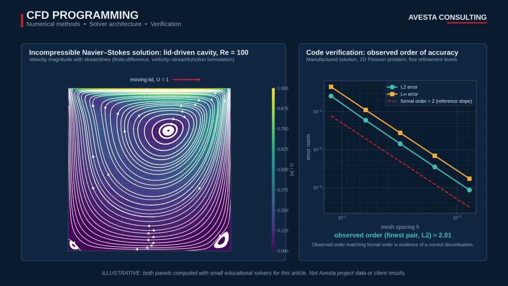
The method of manufactured solutions (MMS) then tests the assembled discretisation. You choose the answer first and make the equations agree with it:
- Choose smooth analytic fields (velocity, pressure, temperature) that are non-trivial enough to make every term of the equations matter. For incompressible flow, choose a divergence-free velocity or add a continuity source.
- Substitute them into the governing equations, with a symbolic tool, to obtain the residual. That residual becomes a source term.
- Add the source terms to the code and set boundary values from the manufactured fields.
- Solve on at least three systematically refined meshes, converging the iterations tightly.
- Compute error norms against the manufactured solution and the observed order, p = ln(e_coarse / e_fine) / ln(r), where r is the refinement ratio.
- Compare p with the formal order of the scheme and investigate any shortfall.
Table 5 shows why this is worth the effort. The numbers are hypothetical, chosen only to show what the test reveals.
| Mesh (relative spacing) | Case A: L2 error in u | Case B: L2 error in u |
| h | 4.0 × 10⁻³ | 4.0 × 10⁻³ |
| h / 2 | 1.0 × 10⁻³ | 2.0 × 10⁻³ |
| h / 4 | 2.5 × 10⁻⁴ | 1.0 × 10⁻³ |
| Observed order | 2.0, 2.0 (matches a second-order scheme) | 1.0, 1.0 (a first-order error is contaminating the solution) |
Table 5. Hypothetical order-of-accuracy results for two versions of a solver with a second-order scheme. Illustrative values only.
Case B could come from, for instance, a first-order boundary treatment. It can look plausible on a contour plot and pass a single benchmark, yet the order test exposes it. The Sandia study by Salari and Knupp found that MMS identifies coding mistakes that affect order of accuracy, and its blind tests also showed categories of mistake it cannot expose.
Know the limits. MMS does not detect errors in terms absent from the manufactured problem. Smooth solutions do not exercise limiters, shocks or discontinuities. If the code and the source terms share the same misunderstanding of the equation, the test passes. And it says nothing about whether the physical model is appropriate or the solver is robust.
Order-of-accuracy and grid-convergence studies
When no exact solution exists, as for a real geometry, you move from code verification to solution verification: estimating the discretisation error in the specific simulation. The widely used procedure of Celik and co-authors (ASME Journal of Fluids Engineering, 2008) uses at least three systematically refined meshes, recommends a refinement ratio above about 1.3, solves for the observed order p, applies Richardson extrapolation, and reports the grid convergence index. For three meshes the fine-grid index uses a safety factor of 1.25:
GCI(fine) = 1.25 · e_a / (r^p − 1), e_a = |(φ₁ − φ₂) / φ₁|
Here φ₁ and φ₂ are the fine- and medium-mesh values of the quantity of interest. The estimate is only meaningful if the solutions are in the asymptotic range and converge monotonically. Refine systematically, holding wall treatment and mesh topology consistent. Separate iteration error from discretisation error. Remember that the index measures discretisation uncertainty only. It does not capture model-form error such as a RANS closure deficiency, and unsteady turbulent flows add statistical uncertainty from finite averaging.
Validate, Profile and Maintain the Solver
Benchmark and experimental validation
Match each reference case to what it can prove:
- Exact solutions (plane Poiseuille and Couette flow, the decaying two-dimensional Taylor–Green vortex, Kovasznay flow) support code verification, because the error is known exactly.
- Numerical benchmarks such as the lid-driven cavity tabulated by Ghia, Ghia and Shin (1982) support comparison, but the reference carries its own discretisation error and is not an exact solution. Agreement with an independent code, as in the Turbulence Modeling Resource, builds confidence as more cases agree.
- Experiments support validation, but only with measured uncertainties, matched conditions and a stated validation domain.
Validation is a separate evidence chain from verification. Our article on thermal design validation walks through test-to-model correlation and acceptance criteria in detail.
Performance, reproducibility and regression tests
Profile before optimising. Sparse matrix–vector products and linear solves are typically limited by memory bandwidth rather than arithmetic. Parallel solvers usually use domain decomposition with halo exchange, and a parallel run should match the serial result within a stated tolerance. Do not expect bitwise identity across process counts: floating-point addition is not associative, so summation order changes the last digits. The same applies when porting to GPUs, and a port should re-run the verification suite.
Make results reproducible by recording the solver version, compiler and flags, library versions, input files and a mesh checksum in every output. Build the regression suite from the ladder: unit tests and small-mesh MMS studies on every commit, benchmark cases nightly, and solution-verification studies on key cases before each release. Store reference values with tolerances rather than exact matches, tag versions used for client work, and note in the changelog any change that alters numerical behaviour.
Reviewing a solver someone else wrote
The same ladder gives a way to assess an unfamiliar solver. Ask for the evidence in Table 6.
| Evidence to request | What good looks like | Red flag |
| Order-of-accuracy results | Observed order matches formal order on three or more meshes for each discretised term set | Only “it converges” or contour screenshots |
| Automated test suite | Runs on every change and includes failure cases | Manual checks only |
| Boundary-condition documentation | Written contract and test for each type | Behaviour known only by reading source |
| Conservation reporting | Global balances reported for each run | Balances never reported |
| Solution-verification practice | GCI or equivalent on key cases; iteration criteria stated | Single-mesh results presented as final |
| Validation scope | Stated validation domain with uncertainties | A generic claim that the code is “validated” |
Table 6. Evidence to request when reviewing a CFD solver.
Limitations to Keep in View
Verification shows the code solves its equations correctly. It does not show that the equations are the right ones, and a perfectly verified solver with an unsuitable turbulence model still carries model-form error that no mesh refinement will remove. On real unstructured meshes, observed order is often below the formal order of the scheme, and the interpretation of that gap takes judgement. Grid-convergence estimates are unreliable when convergence is not monotone or when the solution contains discontinuities.
Data-driven additions raise the same questions. Surrogate models and learned closures inherit the limits of their training data, so they need the same verification and validation discipline as any other component; our article on machine learning in CFD covers where they help.
FAQ
What language is best for CFD programming?
Compiled languages, mainly C++ and Fortran, remain the mainstream for production solvers because of performance and mature parallel libraries. Python with NumPy and SciPy, or Julia, suits prototyping a scheme and writing verification harnesses, and many teams verify a method in a high-level language before porting it. Architecture matters more than language: the separation of operators, boundary conditions and linear algebra described above.
How many meshes do I need for an order-of-accuracy test?
At least three, so you can see a trend rather than a single pair; four or five give more confidence when the coarsest meshes are not yet in the asymptotic range. For MMS, a refinement ratio of two is simple and clear. For grid-convergence studies on real geometry, a ratio above about 1.3 is recommended.
If my solver passes the lid-driven cavity benchmark, is it verified?
No. One benchmark exercises one geometry, one set of boundary conditions and a limited set of terms, and the reference data have their own error. Agreement can also mask compensating errors. Benchmarks sit on the ladder alongside unit tests and MMS, not in place of them.
Building or Reviewing a CFD Model?
If you are developing a solver or custom model, or want an independent review of a numerical method before it informs design decisions, Avesta can discuss the approach. Our advanced simulation services cover CFD including conjugate heat transfer, rotating domains and multiphase flow, and our team’s engineering software development experience supports custom model work. For independent checking against standards and project requirements, see our design verification service. To start, get in touch with a short description of the equations the solver handles and the decisions its results will support.